Introduction to Sampling Methods

Sampling is difficult.

A general sampling method I can think of.

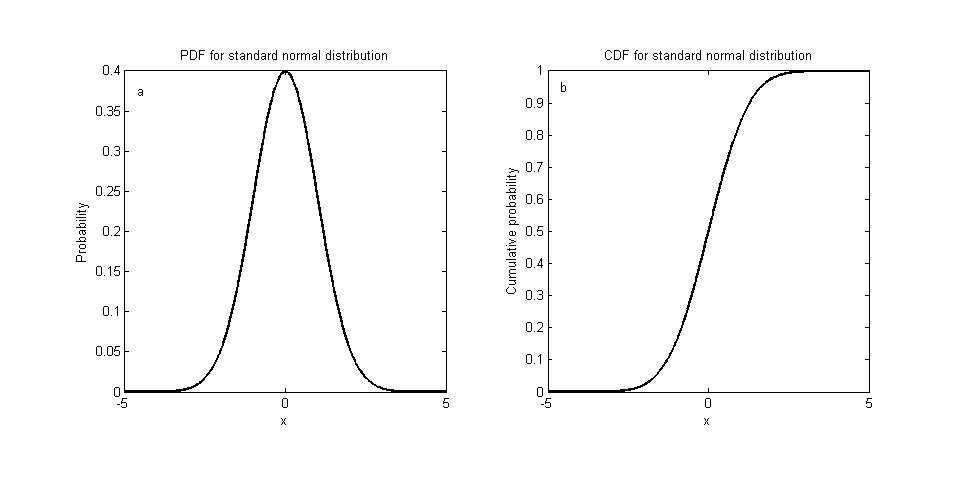
find CDF by integrating PDF from $-\infty$ to x.
find inverse function of CDF.
take a sample from uniform distribution and put the value in the function found.

sampling_by_inverse_cdf

It’s more difficult when it comes to high dimensions.

If it were easy it would have been great

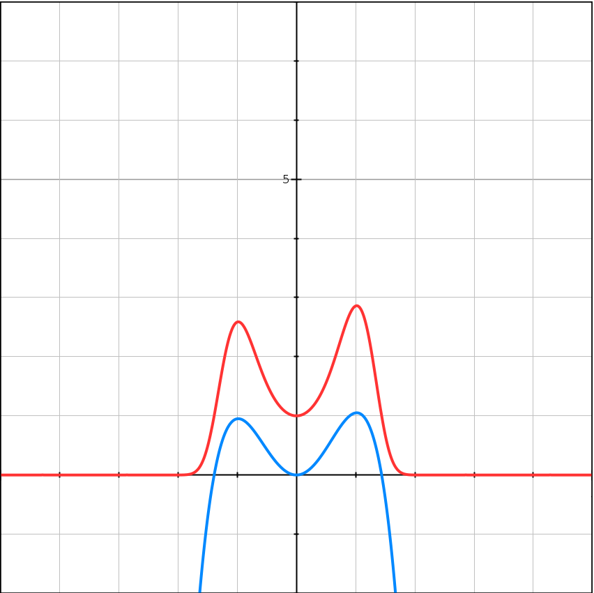
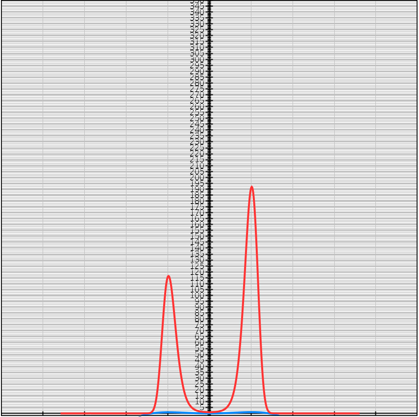
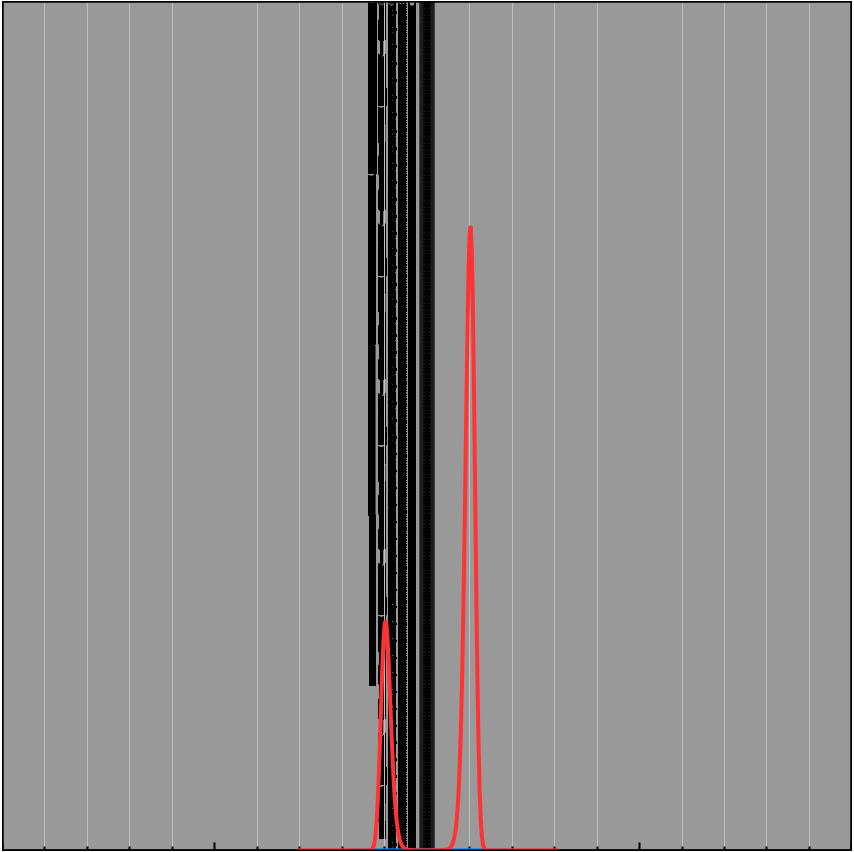
If it were easy to sample always, we could easily find global maximum $\max_x f(x)$ just by taking samples from $\lim_{K \to \infty}e^{Kf(x)}$.

(Frequently, PDF we have is not normalized.)

For example

\[f(x) = -(x-1)^2(x+1)^2 + 1 + 0.05x^3\] \[e^{Kf(x)} = e^{K(-(x-1)^2(x+1)^2 + 1 + 0.05x^3)}\]

$K = 1$	$K = 5$	$K = 10$

Sampling is useful

We can calculate expectation values by sampling.

\[\int f(x)p(x) dx \approx \sum_{i=1}^{N} {f(X_i) \over N}\]

Naive sampling

import numpy as np
import seaborn as sns
import math
from scipy.stats import multivariate_normal

def easy_p(x):
    mean1 = np.array([1, 1])
    cov1 = np.array([[1, 0], [0, 1]])
    mean2 = np.array([3, 4])
    cov2 = np.array([[1, 0], [0, 1]])
    return (4 * multivariate_normal.pdf(x, mean=mean1, cov=cov1) + 1 * multivariate_normal.pdf(x, mean=mean2, cov=cov2))/5

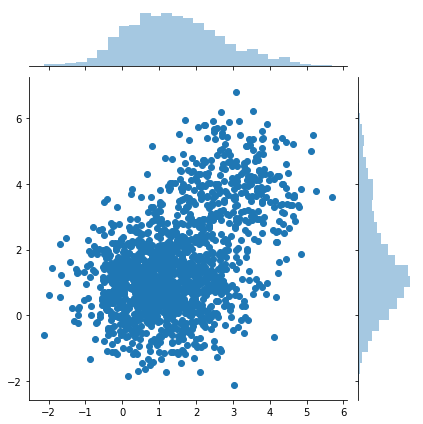
def naive_sample_from_easy_p(iter):
    mean1 = np.array([1, 1])
    cov1 = np.array([[1, 0], [0, 1]])
    mean2 = np.array([3, 4])
    cov2 = np.array([[1, 0], [0, 1]])
    samples = np.zeros((iter, 2))
    for i in range(iter):
        if np.random.rand() < 4/5:
            x_star = multivariate_normal.rvs(mean=mean1, cov=cov1)
        else:
            x_star = multivariate_normal.rvs(mean=mean2, cov=cov2)
        samples[i] = x_star
    return np.array(samples)

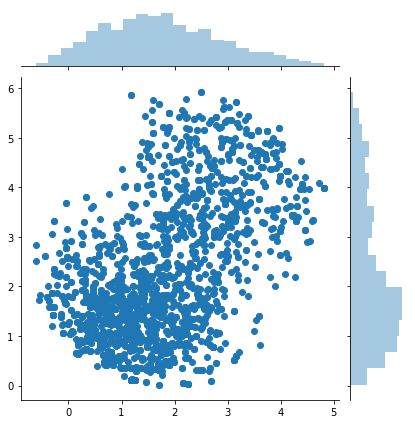
samples = naive_sample_from_easy_p(1500)
sns.jointplot(samples[:, 0], samples[:, 1])
print(samples.shape)

(1500,2)

Rejection sampling

import numpy as np
import seaborn as sns
import math
from scipy.stats import multivariate_normal

def easy_p(x):
    mean1 = np.array([1, 1])
    cov1 = np.array([[1, 0], [0, 1]])
    mean2 = np.array([3, 4])
    cov2 = np.array([[1, 0], [0, 1]])
    return (4 * multivariate_normal.pdf(x, mean=mean1, cov=cov1) + 1 * multivariate_normal.pdf(x, mean=mean2, cov=cov2))/5

def difficult_and_not_normalized_p(x):
    rSquare = (x[0]-2)**2 + (x[1]-3)**2
    return 0 if rSquare > 3**2 else easy_p(x)

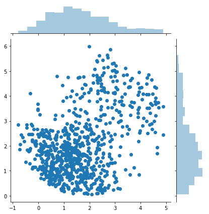
def rejection_sample(f, iter):
    proposal_mean = np.array([2.1, 3.1])
    proposal_cov = np.array([[3, 0],[0, 3]])
    samples = []
    m = 10
    for i in range(iter):
        x_star = multivariate_normal.rvs(mean = proposal_mean, cov = proposal_cov)
        criteria = f(x_star)/(m * multivariate_normal.pdf(x_star, mean = proposal_mean, cov = proposal_cov))
        if criteria > 1:
            # proposal distribution is not enveloping the target distribution
            # increase m
            print(criteria)
        elif np.random.rand() < criteria:
            samples.append(x_star)
    return np.array(samples)

samples = rejection_sample(difficult_and_not_normalized_p, 10000)
sns.jointplot(samples[:, 0], samples[:, 1])
print(samples.shape)

(760, 2)

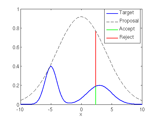
If the proposal distribution is not enveloping the target distribution efficiently

import numpy as np
import seaborn as sns
import math
from scipy.stats import multivariate_normal

def easy_p(x):
    mean1 = np.array([1, 1])
    cov1 = np.array([[1, 0], [0, 1]])
    mean2 = np.array([3, 4])
    cov2 = np.array([[1, 0], [0, 1]])
    return (4 * multivariate_normal.pdf(x, mean=mean1, cov=cov1) + 1 * multivariate_normal.pdf(x, mean=mean2, cov=cov2))/5

def difficult_and_not_normalized_p(x):
    rSquare = (x[0]-2)**2 + (x[1]-3)**2
    return 0 if rSquare > 3**2 else easy_p(x)

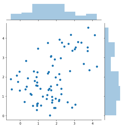
def rejection_sample(f, iter):
    proposal_mean = np.array([3, 3])
    proposal_cov = np.array([[1, 0],[0, 1]])
    samples = []
    m = 500
    for i in range(iter):
        x_star = multivariate_normal.rvs(mean = proposal_mean, cov = proposal_cov)
        criteria = f(x_star)/(m * multivariate_normal.pdf(x_star, mean = proposal_mean, cov = proposal_cov))
        if criteria > 1:
            # proposal distribution is not enveloping the target distribution
            # increase m
            print(criteria)
        elif np.random.rand() < criteria:
            samples.append(x_star)
    return np.array(samples)

samples = rejection_sample(difficult_and_not_normalized_p, 50000)
sns.jointplot(samples[:, 0], samples[:, 1])
print(samples.shape)

(79, 2)

Relationship of sampling methods

sampling methods

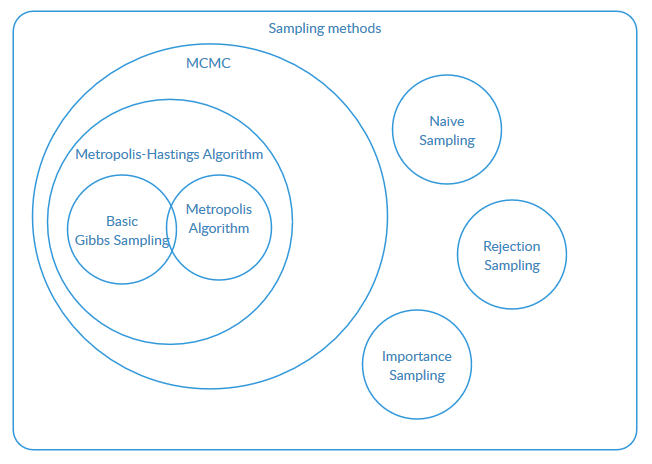
Metropolis-Hastings algorithm

import numpy as np
import seaborn as sns
import math
from scipy.stats import multivariate_normal

def easy_p(x):
    mean1 = np.array([1, 1])
    cov1 = np.array([[1, 0], [0, 1]])
    mean2 = np.array([3, 4])
    cov2 = np.array([[1, 0], [0, 1]])
    return (4 * multivariate_normal.pdf(x, mean=mean1, cov=cov1) + 1 * multivariate_normal.pdf(x, mean=mean2, cov=cov2))/5

def difficult_and_not_normalized_p(x):
    rSquare = (x[0]-2)**2 + (x[1]-3)**2
    return 0 if rSquare > 3**2 else easy_p(x)

def metropolis_hastings(f, iter):
    x = np.array([4., 1.])
    proposal_cov = np.array([[0.5, 0],[0, 0.5]])
    burn_in = 200
    samples = np.zeros((iter, 2))

    for i in range(iter + burn_in):
        x_star = multivariate_normal.rvs(mean=x, cov=proposal_cov)

        a = f(x_star) / f(x)

        # This line can be skipped since the propsed transition probability is symmetric.
        a *= multivariate_normal.pdf(x, mean=x_star, cov=proposal_cov) / multivariate_normal.pdf(x_star, mean=x, cov=proposal_cov)

        if np.random.rand() < a:
            x = x_star
        if i >= burn_in:
            samples[i - burn_in] = x
    return samples

samples = metropolis_hastings(difficult_and_not_normalized_p, 2000)
sns.jointplot(samples[:, 0], samples[:, 1])
print(samples.shape)

(79, 2)

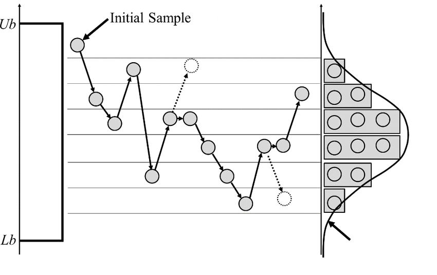
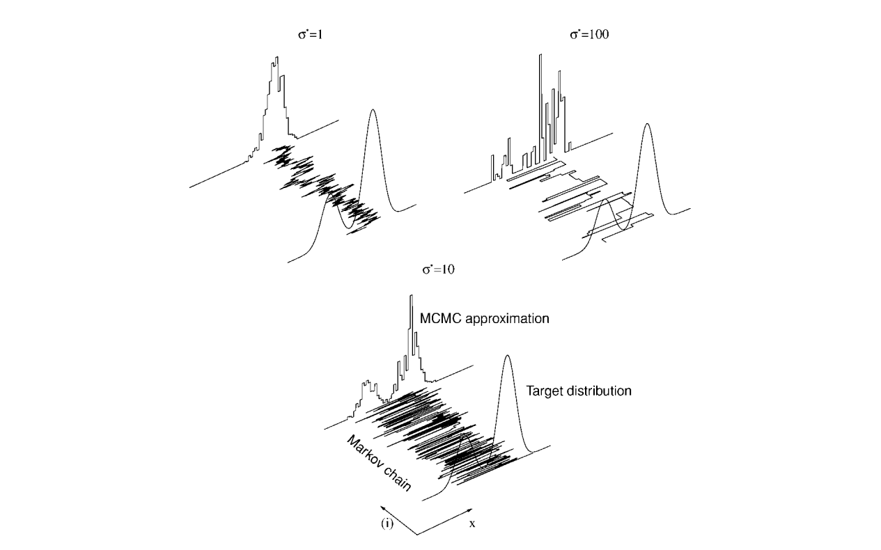
About Markov chain

Try it!

http://markov.yoriz.co.uk/

To be a good Markov chain to sample from

digraph {
    # nodes
    sAccesible [label=accessible]
    sComunicate [label=communicate]
    cIreducible [label=irreducible, shape=box]

    sAperiodic [label=aperiodic]
    sRecurrent [label="positive recurrent"]
    sErgodic [label=ergodic]
    cErgodic [label=ergodic, shape=box, fillcolor=gray, style=filled]

    sDetailedBalance [label="detailed balance"]
    cReversible [label=reversible, shape=box, fillcolor=gray, style=filled]
    cStationaryDistribution [label="has stationary distribution", shape=box]
    cUniquePositiveStationaryDistribution [label="has unique positive stationary distribution", shape=box, fillcolor=lightblue, style=filled]

    and [label="+", shape=circle]

    # edges
    cIreducible -> sComunicate -> sAccesible
    sErgodic -> sAperiodic
    sErgodic -> sRecurrent
    cErgodic -> sErgodic
    cErgodic -> cIreducible
    cReversible -> sDetailedBalance
    cReversible -> cStationaryDistribution
    cReversible -> cIreducible

    cErgodic -> and [style=dashed]
    cStationaryDistribution -> and [style=dashed]
    and -> cUniquePositiveStationaryDistribution
}

A circle is a property of a state.
A box is a property of a Markov chain.

Derivation of MH algorithm

Goal

Design a markov chain that has a stationary distribution $\pi(x)$ such that $\pi(x) = P(x)$ and the stationary distribution is unique.

Propose transition(conditional) probabilities

$P(x^\prime \mid x_t) = g(x^\prime \mid x_t) \cdot A(x^\prime, x_t)$

$g(x^\prime\mid x_t)$ is any proposal distribution chosen.
$A(x^\prime,x_t)=\min \left(1,{\frac {P(x^\prime)}{P(x_{t})}}{\frac {g(x_{t}\mid x^\prime)}{g(x^\prime\mid x_{t})}}\right)$ is acceptance probability.

The markov chain is designed to be reversible

Given $P(x)$ the detailed balance condition can be represented as

$P(x^\prime\mid x)P(x) = P(x\mid x^\prime)P(x^\prime)$ .

It seems to hold always, then the markov chain will have a statinonary distribution. But we need to define such a transition probability. If we let it be composed into a proposal distribution $g(x^\prime \mid x)$ and an acceptance distribution $A(x^\prime, x)$ it can be represented as $P(x^\prime \mid x) = g(x^\prime \mid x)A(x^\prime, x)$. By plugging this into the previous equation, we have.

$ g(x^\prime\mid x) A(x^\prime,x)P(x) = g(x_t, x^\prime) A(x_t, x^\prime)P(x^\prime) $

$ {\frac {A(x^\prime,x)}{A(x,x^\prime)}}={\frac {P(x^\prime)}{P(x)}}{\frac {g(x\mid x^\prime)}{g(x^\prime\mid x)}} $

Now we need to choose $A(x^\prime, x)$ that holds the equality condition above. One common choice is the Meltropolis choice.

$A(x^\prime,x_t)=\min \left(1,{\frac {P(x^\prime)}{P(x_{t})}}{\frac {g(x_{t}\mid x^\prime)}{g(x^\prime\mid x_{t})}}\right)$

Note that either $A(x^\prime,x)$ or $A(x^\prime,x)$ will be 1. Either way, the condition is satisfied.

Show that it is also ergodic

I couldn’t find the proof, but they looks trivial for the markov chain with discrete states.

The markov chain we made is positive recurrent.
- The expected return time of state $i$ is finite.
The markov chain we made is aperiodic.
- We can make infinitely many paths returning to the same state that the number of steps is not periodic with any positive integer which is greater than 1.

By definition it is ergodic.

References

- https://www.youtube.com/playlist?list=PLD0F06AA0D2E8FFBA
- http://www.secmem.org/blog/2019/01/11/mcmc/